欧拉公式 e^jwt=coswt+jsinwt

w=1;
t=0:0.1:20;
f=exp(1j*w*t);%语法问题，写代码最好用1j代替j
x=t;
y=imag(f);
z=real(f);
plot3(x,y,z);
xlabel('时间t');
ylabel('虚部jsinwt');
zlabel('实部coswt');

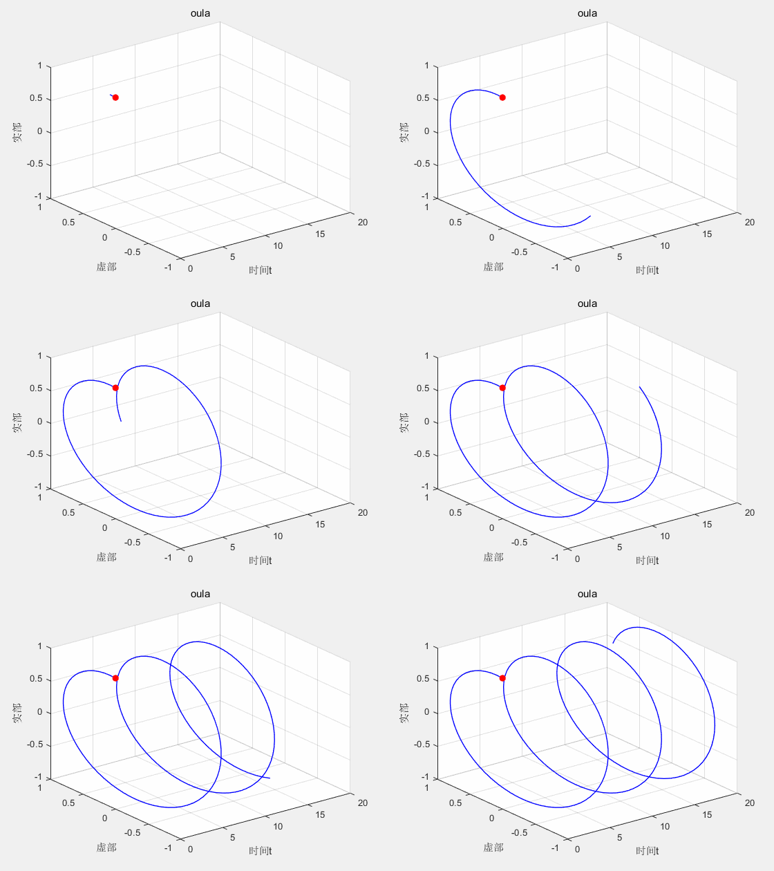
实部为cost图像，f(t)=cost
虚部为sint图像，f(t)=sint
实部和虚部为圆心为0 半径为1 的园
filename='oula.gif';

% 创建数据
t = 0:0.1:20;
x = t;
y = sin(t);
z = cos(t);

% 初始化图形
figure;
h = plot3(x(1), y(1), z(1), 'b-', 'LineWidth', 1);
hold on;
scatter3(x(1), y(1), z(1), 50, 'r', 'filled');
xlabel('时间t');
ylabel('虚部');
zlabel('实部');
title('oula');
grid on;
axis([0 20 -1 1 -1 1]);

% 动态绘制
for i = 2:length(t)
set(h, 'XData', x(1:i), 'YData', y(1:i), 'ZData', z(1:i));
drawnow;

frame = getframe(gcf);
im = frame2im(frame);
[imind, cm] = rgb2ind(im, 256);

% 写入GIF文件

if i == 2
imwrite(imind, cm, filename, 'gif', 'Loopcount', inf, 'DelayTime', 0.1);
else
imwrite(imind, cm, filename, 'gif', 'WriteMode', 'append', 'DelayTime', 0.1);
end

% 控制速度
pause(0.05);
end

傅里叶变换

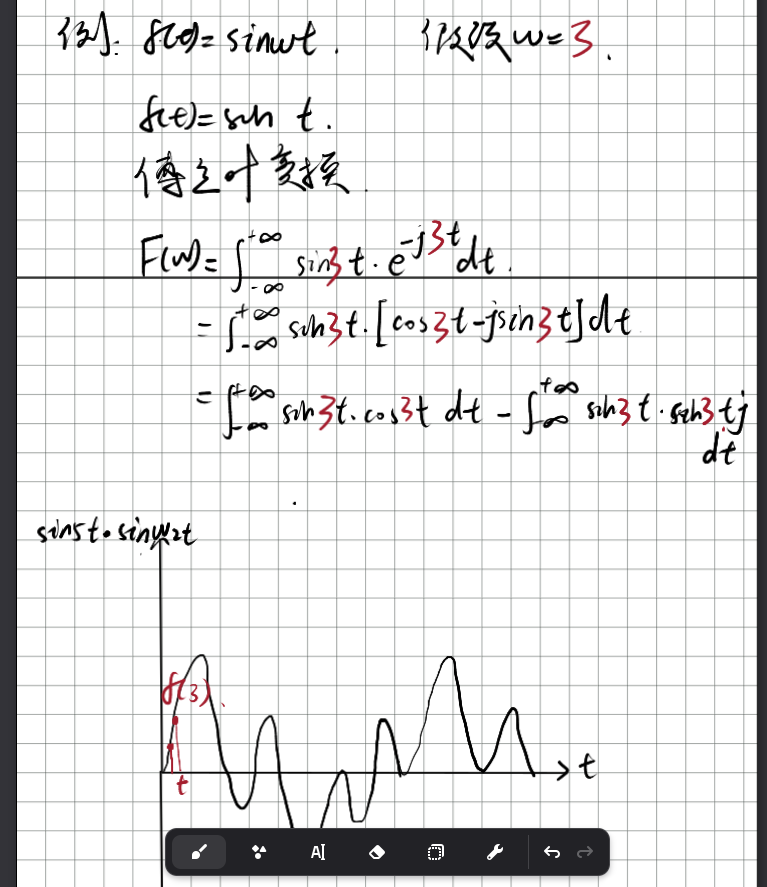
核心思想是将复杂的波形分解成一系列简单的正弦波的叠加

clear
clc

t=0:0.01:20;
w1=3;
w2=0.1:0.1:5;
clf;

for i=1:length(t)
clf;
f1=sin(w1*t);
for j=1:length(w2)
        f2=sin(w2(j)*t);
        subplot(3,1,1);
        plot(t,f2);
        yline(0, '--', 'Color', 'black', 'LineWidth', 1); % 红色虚线，线宽1.5
        legend('sin(5t)','sin(wt)');
        pause(0.01);
        cla

        subplot(3,1,1);
        plot(t,f1);
        yline(0, '--', 'Color', 'black', 'LineWidth', 1); % 红色虚线，线宽1.5
        hold on;
        xlabel('时间t');
        ylabel('sinwt');
        title(sprintf('w2 = %d', w2(j)));
        
        subplot(3,1,2);
        f3=f1.*f2;
        plot(t,f3);
        yline(0, '--', 'Color', 'black', 'LineWidth', 1); % 红色虚线，线宽1.5
        xlabel('时间t');
        ylabel('f(t)');
        title('f(t)');

        subplot(3,1,3);
        axis([0 50 -5 10]);
        g=@(t) sin(w1*t).*sin(w2(j)*t);
        q=integral(g,0,20);
        disp(q);
    
        hold on;
        scatter(j,q,10,'red','filled');
        yline(0, '--', 'Color', 'black', 'LineWidth', 1); % 红色虚线，线宽1.5
        xlabel('时间t');
        ylabel('积分');
        title('积分');
    end
end

若未知信号的初始相位为90°，

傅里叶变换的实部表示未知信号与cos信号的相关度，虚部表示未知信号与sin信号的相关度
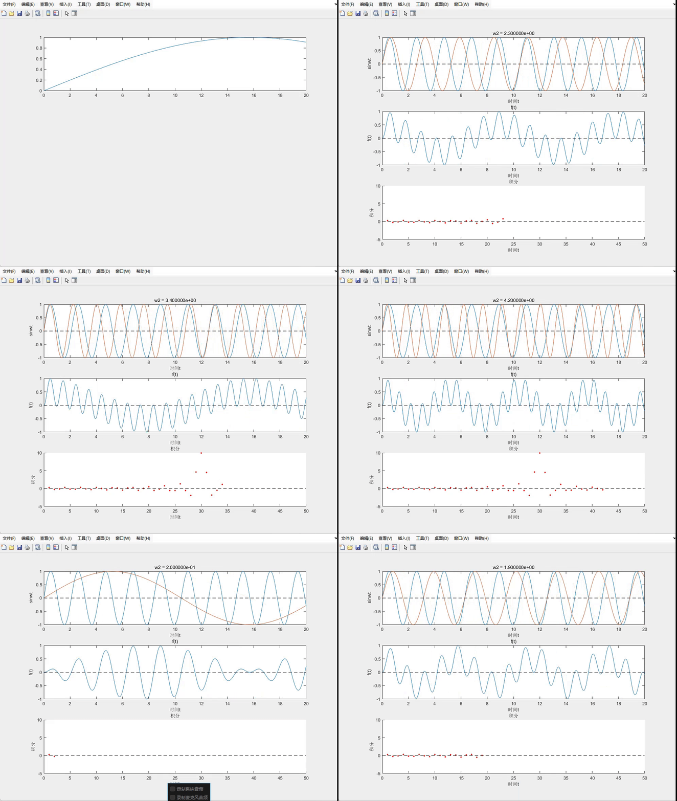
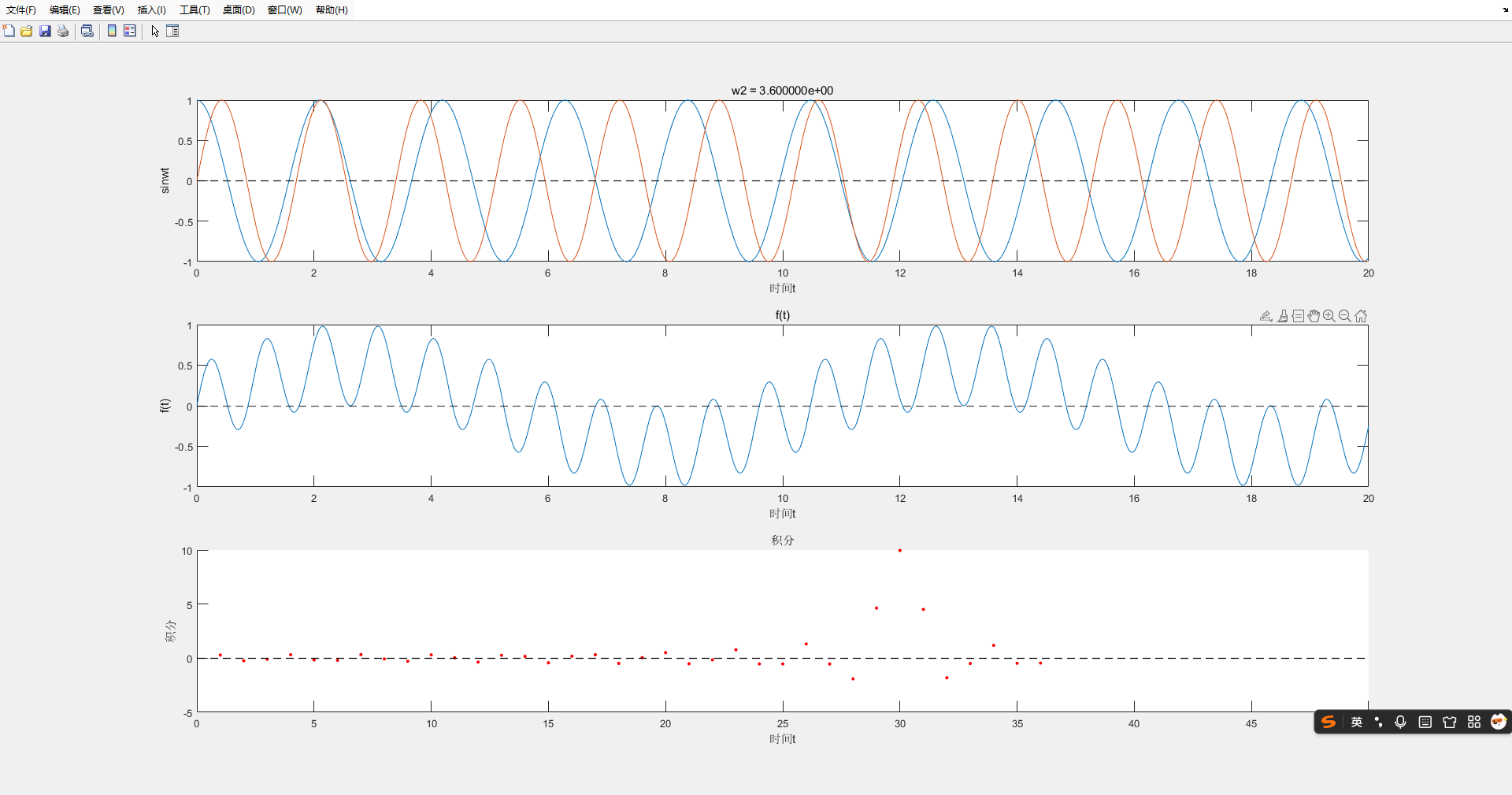
当未知信号与基信号频率相同时，他们乘积的积分达到了最大。而这个积分最终的图像是不是就很像信号经过傅里叶变换后的频域图像，就是用各种频率的基信号与未知信号做对比，看看哪个频率的基信号与未知信号最像！！！，而这个对比的方法，用数学来描述就是先相乘后积分
左边为sin3tsinwt，为傅里叶变换的虚部，右边为sin3tcoswt,为傅里叶变换的实部

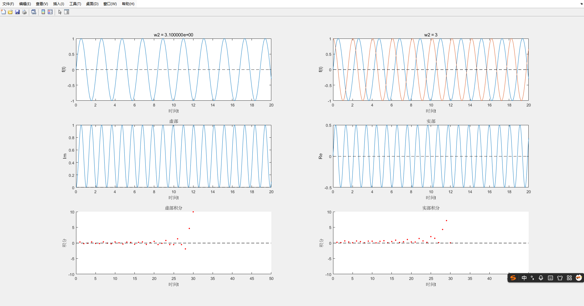
当w提增到目标的w=3时，两个sin波形重合，想乘后均大于0，此时对其虚部的积分达到最大值
其实部为sin3t*coswt，积分值则不同，当w遍历到3时，和未知信号w=3达到同频，上下半轴抵消，其积分为0
clear
clc

filename='fly.gif';
t=0:0.01:20;
w1=3;
w2=0.1:0.1:5;

for i=1:length(t)
    clf;
    f1=sin(w1*t);
    p1=cos(w1*t);

    for j=1:length(w2)
        f2=sin(w2(j)*t);      %sinwt
        subplot(3,2,1);
        yline(0, '--', 'Color', 'black', 'LineWidth', 1); % 红色虚线，线宽1.5
        plot(t,f2);
        pause(0.001);
        cla

        subplot(3,2,1);     %sin3t
        plot(t,f1);
        yline(0, '--', 'Color', 'black', 'LineWidth', 1); % 红色虚线，线宽1.5
        hold on;
        xlabel('时间t');
        ylabel('f(t)');
        title(sprintf('w2 = %d', w2(j)));

        p2=cos(w2(j)*t);    %coswt
        subplot(3,2,2);
        yline(0, '--', 'Color', 'black', 'LineWidth', 1); % 红色虚线，线宽1.5
        plot(t,p2);

        pause(0.001);
        cla

        subplot(3,2,2);    %sin3t
        plot(t,f1);
        yline(0, '--', 'Color', 'black', 'LineWidth', 1); % 红色虚线，线宽1.5
        hold on;
        xlabel('时间t');
        ylabel('f(t)');
        title(sprintf('w2 = %d', w2(j)));


        subplot(3,2,3);  %虚部sin3t*sinwt
        f3=f1.*f2;
        plot(t,f3);
        yline(0, '--', 'Color', 'black', 'LineWidth', 1); % 红色虚线，线宽1.5
        xlabel('时间t');
        ylabel('Im');
        title('虚部');

        subplot(3,2,4);  %实部sin3t*coswt
        p3=f1.*p2;
        plot(t,p3);
        yline(0, '--', 'Color', 'black', 'LineWidth', 1); % 红色虚线，线宽1.5
        xlabel('时间t');
        ylabel('Re');
        title('实部');

        subplot(3,2,5);     %虚部积分
        axis([0 50 -10 10]);
        g=@(t) sin(w1*t).*sin(w2(j)*t);
        q=integral(g,0,20);
        disp(q);

        hold on;
        scatter(j,q,10,'red','filled');
        yline(0, '--', 'Color', 'black', 'LineWidth', 1); % 红色虚线，线宽1.5
        xlabel('时间t');
        ylabel('积分');
        title('虚部积分');

        subplot(3,2,6);     %实部积分
        axis([0 50 -10 10]);
        g=@(t) sin(w1*t).*cos(w2(j)*t);
        q=integral(g,0,20);
        disp(q);

        hold on;
        scatter(j,q,10,'red','filled');
        yline(0, '--', 'Color', 'black', 'LineWidth', 1); % 红色虚线，线宽1.5
        xlabel('时间t');
        ylabel('积分');
        title('实部积分');

    end

end

对实部和虚部积分后的值进行开根号

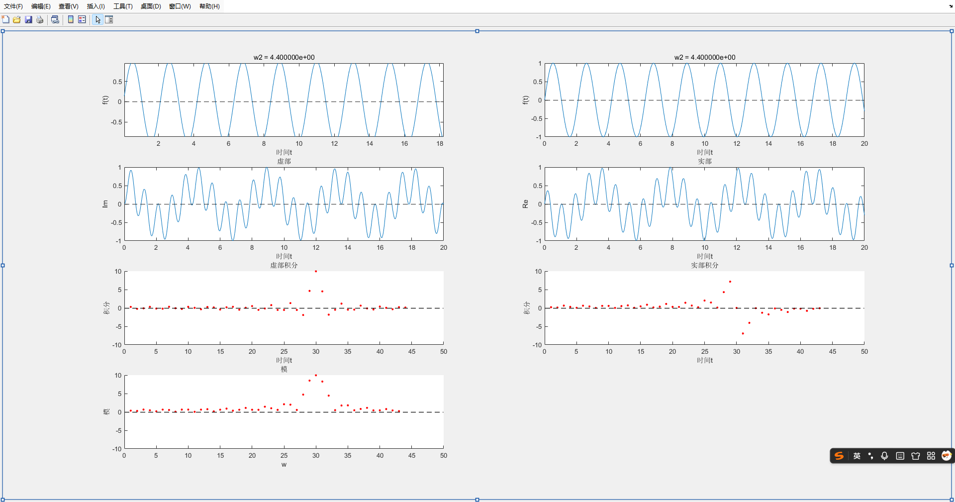
subplot(4,2,7); %实部积分
axis([0 50 -10 10]);
s=sqrt((q1^2)+(q22));
hold on;
scatter(j,s,10,'red','filled');
yline(0, '--', 'Color', 'black', 'LineWidth', 1); % 红色虚线，线宽1.5
xlabel('w');
ylabel('模');
title('模');
可以看出目标信号的频率成分

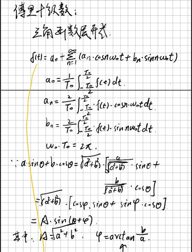
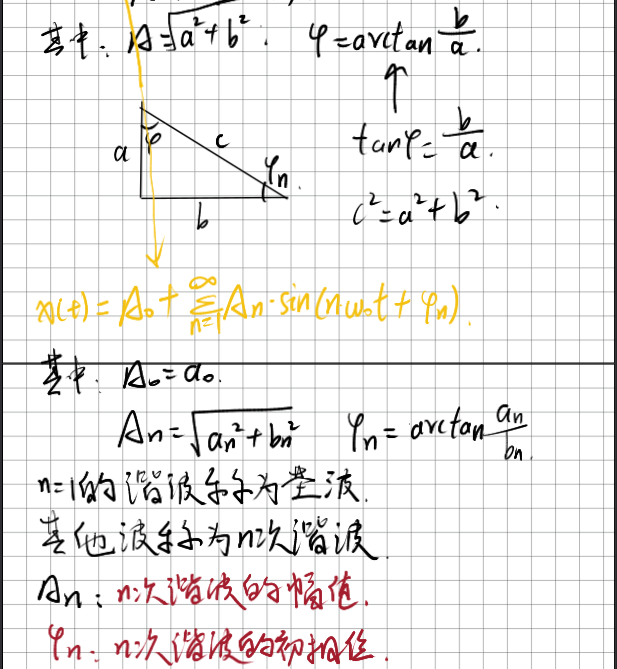
傅里叶级数

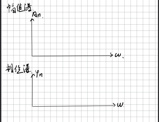
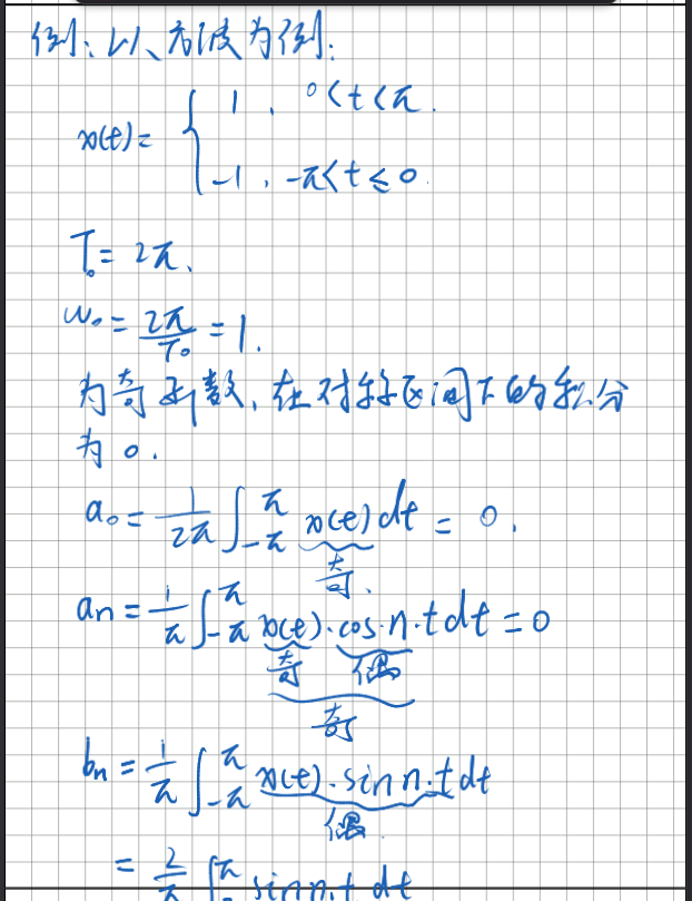
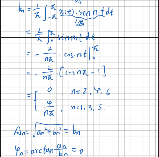
clear
clc

T0=2*pi;
w0=(2*pi)/T0;

n=1:1:30;

% 基本方波绘制
t = 0:0.001:30;        % 时间向量，从0到4秒，步长0.001
g=square(t);

figure;
subplot(3,1,1);
plot(t, g, 'LineWidth', 2);
title('基本方波');
xlabel('时间 (s)');
ylabel('幅度');
ylim([-1.5 1.5]);
grid on;

for i= 1:length(n)
    y = @(t) square(t);   % 生成频率为1Hz的方波
    y2=@(t) square(t).*cos(i*t);
    y3=@(t) square(t).*sin(i*t);


    a0=(1/2*pi).*integral(y,-pi,pi);


    an=(1/pi).*integral(y2,-pi,pi);
    bn=(1/pi).*integral(y3,-pi,pi);

    An=sqrt(an^2+bn^2);

    fann=atan2(0,0);


    subplot(3,1,2);
    hold on
    scatter(n(i),An,10,'red','filled');
    yline(0, '--', 'Color', 'black', 'LineWidth', 1); % 红色虚线，线宽1.5
    xlabel('n');
    ylabel('An');
    title('幅值');

    subplot(3,1,3);
    hold on
    scatter(n(i),fann,10,'red','filled');
    yline(0, '--', 'Color', 'black', 'LineWidth', 1); % 红色虚线，线宽1.5
    xlabel('n');
    ylabel('fann');
    title('相位');

end

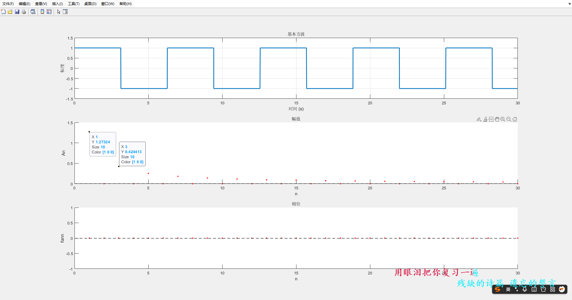
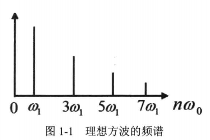
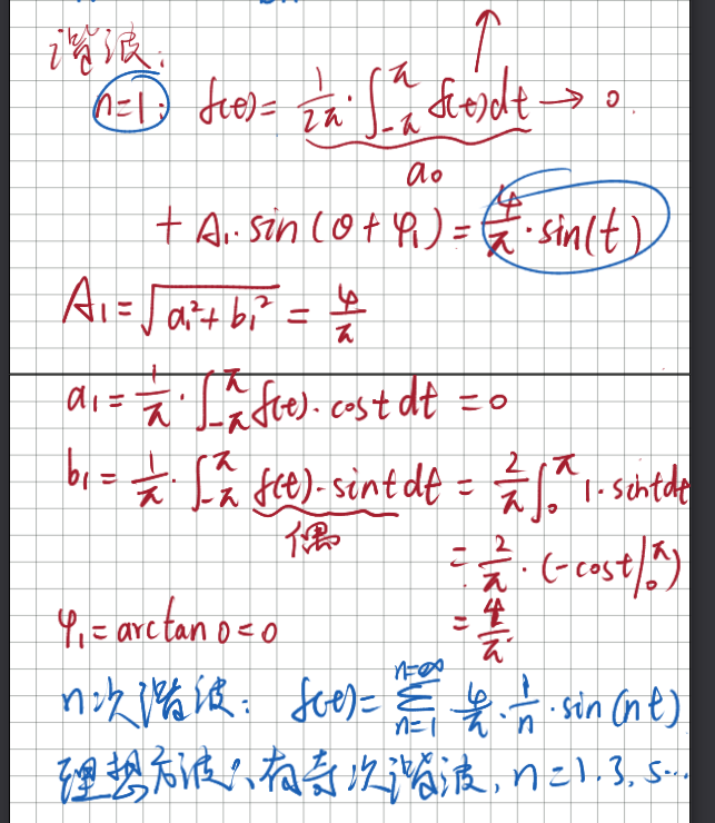
- n次谐波

clear
clc

T0=2*pi;
w0=(2*pi)/T0;

n=1:2:29;

% 基本方波绘制
t = 0:0.001:10;        % 时间向量，从0到4秒，步长0.001
g=square(t);


figure;
plot(t, g, 'LineWidth', 2);
hold on;


title('基本方波');
xlabel('时间 (s)');
ylabel('幅度');
ylim([-1.5 1.5]);
for i=1:length(n)

    f=(4/(pi*n(i))*sin(n(i)*t));
    plot(t,f);

end
grid on;

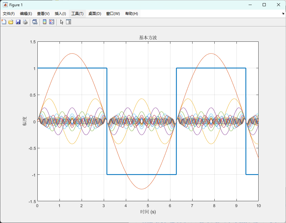
• 理想方波的1~29次谐波叠加

  clear
  clc

  T0=2pi;
  w0=(2pi)/T0;

  n=1:2:29;

  % 基本方波绘制
  t = 0:0.001:10; % 时间向量，从0到4秒，步长0.001
  g=square(t);

  figure;
  subplot(2,1,1);
  plot(t, g, 'LineWidth', 2);
  hold on;

  title('基本方波及其谐波');
  xlabel('时间 (s)');
  ylabel('幅度');
  ylim([-1.5 1.5]);
  for i=1:length(n)

  f(i,:)=(4/(pi*n(i))*sin(n(i)*t));
  plot(t,f);
  end

  for j=1:length(t)
  fs(:,j)=sum(f(:,j));
  end

  subplot(2,1,2);

  plot(t, g, 'LineWidth', 2);
  hold on;
  plot(t,fs);
  title('基本方波及谐波叠加');
  xlabel('时间 (s)');
  ylabel('幅度');
  ylim([-1.5 1.5]);
  grid on;

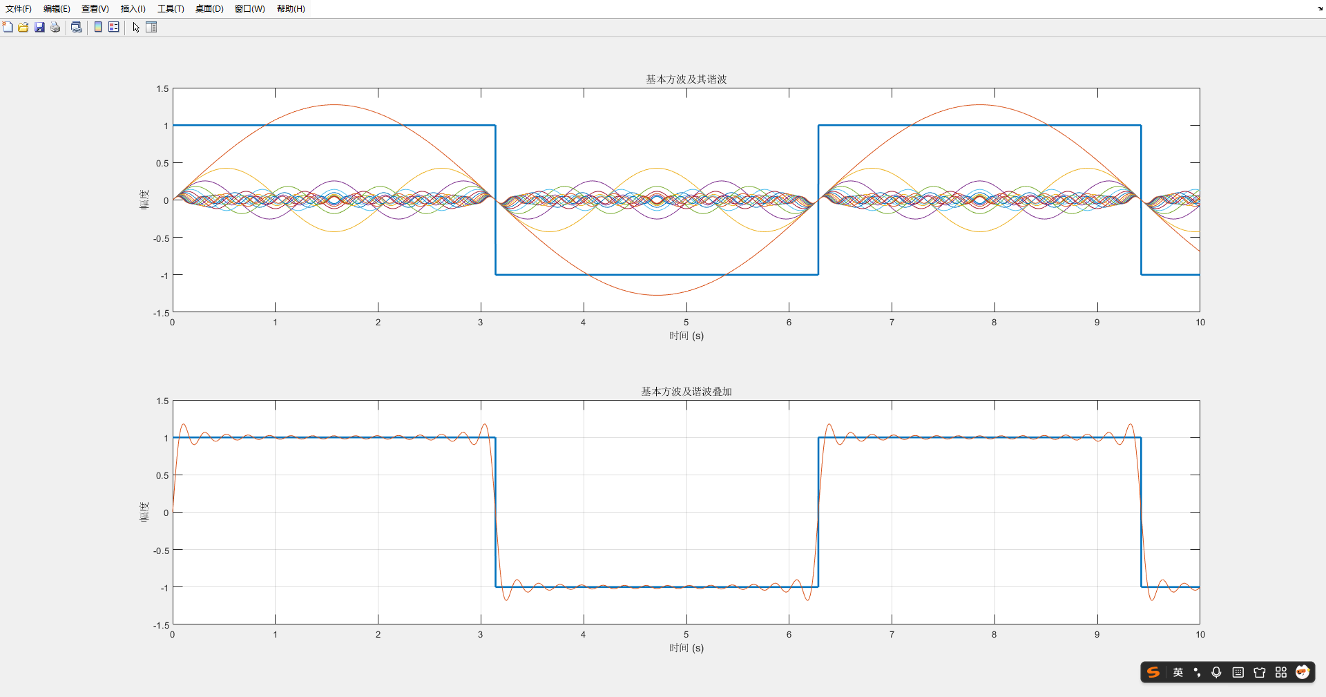
下图为叠加1、3、5次谐波的对比图

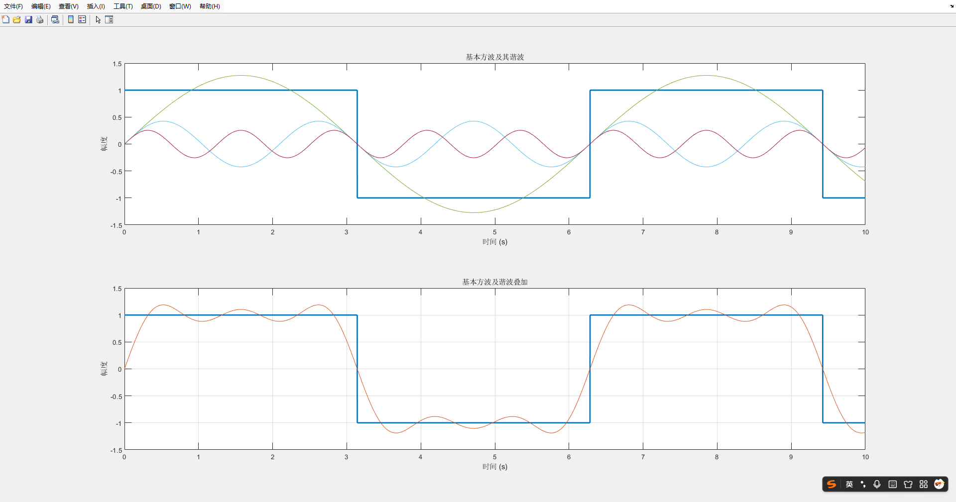
可知：高频分量越多（既是频率，也指幅度），信号的上升沿越陡，高频谐波主要影响信号边沿时间，低频的分量影响幅度。